In the last article, I discussed the concept of feature engineering as comprising two components with the first component being the ability to create and derive meaningful variables in the analytical file which is used as the source information in the development of any predictive analytics solution. Within this first component, access to data has grown exponentially with data scientists now being able to use semi-structured and unstructured data as data inputs. Although the ETL process for this type of data requires new technical skills to essentially structure this data, the intensive data science work in creating and deriving variables still adheres to the same disciplines that have been used for the last 30 years.
Meanwhile, the second component looks at tools and techniques that are used against the analytical file in reducing or filtering out the number of fields which will be analyzed by the more advanced mathematical routines. As the data science industry matures as a discipline, new tools continue to emerge within the industry that facilitate this process for the practitioner Many schools of thought emanate from this discussion in how to best filter or reduce the variable inputs for modelling.. One of the most commonly discussed techniques is the use of PCA (principle components analysis), which is the commonly used version of factor analysis. Although PCA and factor analysis is a great data reduction technique, it is unsupervised implying that this information filter occurs without the use of any information from the target variable. Let’s take a look at an example.
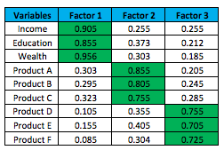
The above example is simplistic in order to better demonstrate the benefits of factor analysis in its use as a data or variable reduction technique. In the real world though, this technique is applied against hundreds of thousands of variables. Yet, in developing predictive models, the question remains as to whether this technique is really optimal in the selection of variables. Factor analysis being an unsupervised technique is selecting variables based on a given factor’s variation relative to all the variation on the data. But shouldn’t techniques be used that look at variation of the data but with respect to the target variable’s overall variation. In other words, the selection of variables should be supervised based on the target variable we are trying to predict. Techniques such as correlation analysis and/or decision trees are examples of this supervised approach.
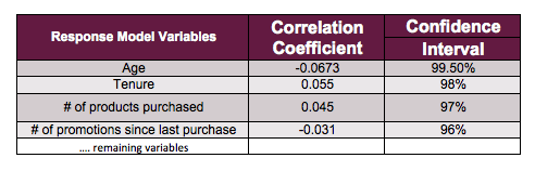
Once our analytical file with the many independent variables and dependent variable has been created, correlation analysis can be conducted to rank order variables based on the absolute value of the correlation coefficient. In developing a typical response model, the analyst might run several hundred variables to be correlated against response. The output would then indicate the top variables which are significant against response albeit in a uni-variate manner. Selecting the “top” variables is where the “art of data science” comes into play. In working with data sets that encompass hundreds of thousands of records, most of the several hundred variables will be statistically significant at a 95% level. But the variables are rank-ordered and could be used to select the top 50-100 variables which would be considered in the more robust multivariate routines. See example below for a typical response model which lists the top 4 variables as correlated against response.
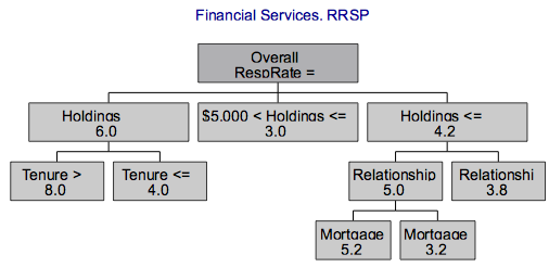
The use of decision trees is another technique which can be used to detect if there are key interactions between variables. Although decision trees in many cases are used to actually create models, one can also apply decision trees against the top variables(top 20 variables) as determined from correlation. The critical piece of knowledge arising from the use of decision trees as opposed to correlation analysis are the identification of key interaction variables. For example, we might discover that age and gender such as males under 25 years represent a key interaction in predicting auto claim losses. In a response model, customer tenure and where they live might be another interaction variable in predicting response. In our example below which is trying to optimize response in an RRSP model, we see the interaction variables between financial holdings and tenure vs. financial holdings and relationships and mortgage.
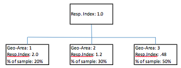
Besides the determination of interaction variables, another capability of decision trees is the ability to group very sparse data into groups. For example, zip codes in the U.S. or postal codes in Canada represent very fine levels of geography that typically would contain a small proportion of individuals that reside in this area relative to those other records not residing in the area. Developing a binary variable at this level would be a meaningless exercise as in most cases the proportion of individuals residing in the area relative to those records not living in the area would be very small.(typically well under 5%). There is simply no way that a pattern or trend can be determined with < 5% of the individuals actually residing in that area. With decision- trees, these geo-area levels can then be grouped to larger geo-areas such that larger geo-area groupings now contain significant proportion of records(20% or higher). Here, the grouping determination is supervised in that the target variable or variable being modelled is optimizing the grouping categories based on how they impact the target variable. See example below.
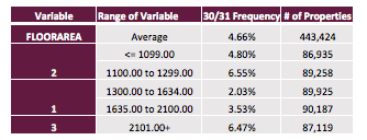
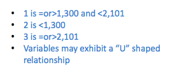
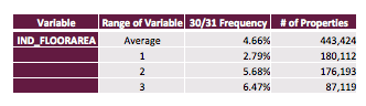
Another example of filtering out variables is the use of exploratory data analysis techniques which enable the practitioner to identify the optimum transformation of a given variable but eliminate the original variable with its source information. Listed below is one example which examines the impact of the floor area of properties and its impact on frequency of claims on properties. In the example here, we observe that the trend tends to be bi modal rather than linear.
Both components (derivation of new variables and filtering- out variables) of feature engineering represent the most labor-intensive phase of the predictive analytics process. Yet, most practitioners consider feature engineering as being most important within the predictive analytics process. Using the analogy of cooking, one can compare feature engineering as the determination of the key inputs into a meal while the determination of the right temperature for cooking can be compared to using the right mathematical technique for predictive models. But as in predictive analytics, feature engineering is the most critical stage in cooking which is reinforced by the level of content in cookbooks that are devoted to inputs and ingredients.
Richard Boire, B.Sc. (McGill), MBA (Concordia), is the founding partner at the Boire Filler Group, a nationally recognized expert in the database and data analytical industry and is among the top experts in this field in Canada, with unique expertise and background experience. Boire Filler Group was recently acquired by Environics Analytics where I am currently senior vice-president.
Mr. Boire’s mathematical and technical expertise is complimented by experience working at and with clients who work in the B2C and B2B environments. He previously worked at and with Clients such as: Reader’s Digest, American Express, Loyalty Group, and Petro-Canada among many to establish his top notch credentials.
After 12 years of progressive data mining and analytical experience, Mr. Boire established his own consulting company – Boire Direct Marketing in 1994. He writes numerous articles for industry publications, is a well-sought after speaker on data mining, and works closely with the Canadian Marketing Association on a number of areas including Education and the Database and Technology councils. He is currently the Chair of Predictive Analytics World Toronto.