Last month, I discussed the importance of variable selection as a key component of the modelling process. We examined three techniques: factor analysis, correlation analysis, and clustering. This month, we will explore CHAID/Decision Tree, Exploratory Data Analysis(EDA), and Stepwise Regression as other techniques in selecting the appropriate variables for a given model.
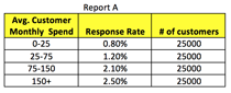
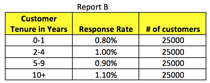
EDA presents a more visual rather than statistical perspective of how a given input variable impacts the target variable. EDA reports depict how a given input variable is trending against the target variable. The practitioner can then select those variables which visually exhibit a trend and exclude those variables which do not exhibit any trend. Listed below are two examples of simple EDA reports with Report A depicting a positive trend between response and customer spend while Report B displays no trend between response and customer tenure.
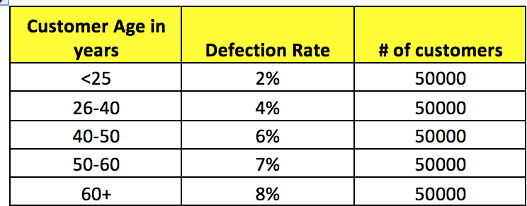
Within a given predictive analytics exercise, EDA’s would be conducted on every variable in the analytical file. Typically, these reports are produced after the correlation reports. They in some respects support the findings of the correlation report. For example, if there is a positive correlation coefficient between defection and age, then the EDA would visually demonstrate that older people are more likely to defect.
EDA reports help to limit the “black box” of predictive analytics by providing the business with user friendly reports that help in their understanding of all the potential modelling inputs.
Income % of Customers Response Rate Income >40
Yet, EDA reports also provide valuable information in terms of creating binned variables particularly for continuous variables. For example, are there certain continuous variables where a simple yes/no binary variable will suffice versus leaving the variable in its raw continuous form.
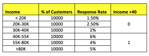
Perhaps, the continuous variable in another example is better represented by a more ordinal approach as seen below.
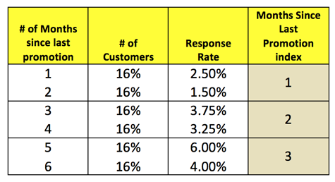
In fact, algorithms exist to optimize what these bins should be versus a target variable. But in any event, the more mathematical approach to optimal binning particularly with variables that end up in the final model should still be depicted through an EDA.
Another more direct mathematical approach to variable selection is the use of decision trees. Here instead of using decision trees such as CHAID or CART to actually create the model, we use the decision tree to group variable outcomes or values together into optimal bins. This is particularly useful for character format variables that have too many values. Typically, binary variables(0/1) variables are created for each outcome. With many outcomes, these binary variables can become too sparse in the sense that there too few 1’s and too many 0’s for these binary variables to have any statistical rigor. Through this approach, the many data outcomes are grouped into broader categories that can now become statistically significant in a modelling exercise. See example below.
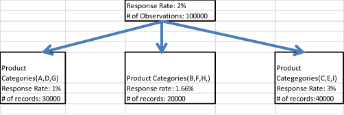
In the above example, nine product categories have been grouped into three product nodes from the decision-tree routine. In this case, the user creates a new ordinal variable with 3 outcomes(1 if category A,D, or G, 2 if category B,F,H or 3 if category C,E, or I). These ordinal category levels are determined mathematically based on the node being statistically significant versus the target variable. This is another example of supervised learning being used to create new variables.
Many practical examples exist such as grouping of detailed postal zip codes into broader geographic areas. For retailers, it could be the ability to group even more detailed level product SKU’s into broader product categories. The creation of binary variables for each of the many product variables would in all likelihood not yield any significant variable in a final model due to the sparseness of data(too few 1’s and too many. But the ability to group products together into broader product categories provides more opportunity that these inputs will become significant in a modelling exercise.
At this point, we now have an input or analytical file with all those variables that have been deemed analytically useful. Through pre-modelling analysis, we have both filtered and added variables to the analytical file. We are now at the stage of using multivariate techniques to further reduce our variable set as it is not unusual to have 100 variables that could be considered as potential model variables. One approach is to use a series of simple multiple regression stepwise routines where 10-20 variables are run in one given stepwise routine. The surviving variables of each stepwise regression are then run against the surviving variables of the other stepwise routines. Each subsequent stepwise procedure should contain no more than 20 variables. Running stepwise procedures with too many variables(i.e. 100) may in fact cause variables to be dropped due to multicollinearity. Some of these variables if used as a smaller subset in a stepwise routine could survive in a final model as they explain a component of the variation that is not being explained by the other model variables. By running one big stepwise routine against all 100 variables, we may exclude certain variables which might otherwise have survived if we adopted the approach of using a series of stepwise routines. The key in using a series of stepwise routines is to minimize the loss of potential information thereby providing the potential of building a stronger model.
Using a series of stepwise routines provides the final filter in building models using multiple regression or logistic regression or in decision trees. More advanced techniques such as neural nets lend themselves to using many more variables with a final set of variables which may typically range from 5 to 10 key variables. The disadvantage here is that the model becomes more of a “blackbox” as it becomes extremely difficult to communicate the key insights from these variables as many of the relationships are non linear in nature. Yet, if the neural net delivers consistent results, explanation may not matter as much. Practical examples of where neural net models are more rigorously employed is in the area of fraud detection due to their increased level of performance amongst these type of models when compared to the linear or log-linear models.
The discussion above looks at variable selection based on learning from prior practical experience. Obviously, each data scientist will have their own accumulated experiences. Ultimately, it is these experiences that provide the art in selecting variables for a given modelling exercise. Yet, as often been stated before, it is this complementation of art and science that is the real key to building successful solutions.
By: Richard Boire, Founding Partner, Boire Filler Group