
The Employee Cost Curve
It is simple enough to document the hard costs that make up the initial stages of employee life-cycle. This section will walk through the major cost areas, but the specifics will depend on the role at hand. We don’t suggest modeling “soft costs” such as morale or engagement, as they are easy to manipulate and difficult to defend.
Typically a small number of meetings and accounting queries are all that is needed to put a simple aggregate together. It is a good practice to assemble the costs in a shared spreadsheet for the involved parties’ approval.
Recruiting Costs
Human Resources spends a great deal of time and effort to fill one position. Typically a recruiter will screen, interview, and reject many candidates before finding the right person. What does this cost?
Such costs often include the following:
In addition, managers and staff spend time interviewing candidates. This is usually well documented, consisting of phone or video interviews, panel interviews, and final individual interviews. They cost money, including:
These costs are surprisingly consistent. Some items, like drug tests, have fixed costs. HR works hard to keep the hiring funnel efficient and full. There is usually a fixed set of job fairs, advertising and job board usage per year.
All of these costs get aggregated and averaged for the role, and applied to the first day of a new hire’s job. It is not unusual for this acquisition cost to be quite high.
On-Boarding Costs
What are the costs to bring one employee on board? Some companies have regular orientation events to welcome new hires.
Such costs often include the following:
Employee salary typically starts during orientation. As above, these costs simply go into the spreadsheet on the proper day.
If termination costs are significant, you may want to include them here on day 1. Essentially, we are accounting for the prior employee’s termination.
Training Costs
What are the costs to train one employee?
Such costs often include the following, averaged per hire:
How many days, weeks, or months is the training? Is there a test at the end, and if so, how many pass the test? Is the new employee paid at full salary during the training?
As before, these costs are relatively fixed and can be filled into the spreadsheet.
On the Job Learning
Even after training, employees are not fully productive. The actual ramp-up is not a cost, but part of performance. We will cover that in the next section – it is important to not double-count.
But during ramp-up, most new employees consume the attention of managers and peers. Often this is the expected procedure, and can be modeled into the costs like everything else. For example, a bank supervisor may watch every transaction for a new bank teller, until milestones are met.
Where peer attention is significant and structural, it makes sense to build simple rules to factor it in. For example, a model may include 20% more of a supervisor’s time (and therefore salary) for the first month. Again, we roll this into the model, day by day.
Base Salary, Benefits and Infrastructure
In most large organizations, employee salaries for a role fall within a reasonably tight band. In an entry-level position, such as a call center, the first-year salary may be completely standardized. Even in positions with large individual variances, the long-term patterns are often quite stable. The goal is to build a reasonable model of the salary for one new employee in this role. If there is a probationary salary, simply model it in.
Sales commissions and other bonuses are performance-based. They can be included here, or deducted from performance numbers in the next section. Commissions can be dominant in a role, or a secondary effect. The important thing is to be consistent, and not double-count costs vs. performance.
Add in other fixed, ongoing costs for the employee, such as health insurance or other benefits, at the time that they start. If benefits start later in the cycle, simply model it in.
Some infrastructure is appropriate for inclusion – incremental ongoing fees, such as electricity or building usage. However, do not include infrastructure that is reused when the employee is replaced – for example a computer or desk will be used by a replacement employee.
Once the employee is at full productivity, costs are typically limited to salary, benefits, and infrastructure. For long-term roles, we model in raises and bonuses. When an employee is promoted, they have effectively left the role of this analysis.
Summing up the Cost Curve
The result is a list of daily costs for having an employee on board in this role. If they end up terminating, the costs will stop. But, this metric does not handle terminations – that comes later.
It isn’t necessary to cover edge cases, like lawsuits or medical emergencies. These are exceptions – a distraction from the overall patterns that will emerge.
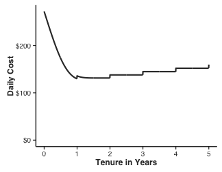
Figure 2. The Cost Curve
A typical curve for an entry-level role may resemble the above – high spikes at the onset, followed by a slow stair-step pattern.
The Employee Performance Curve
Employee Performance is the amount that an individual contributes to corporate revenue. We use this word because “Benefit” can become confused with “Benefits.” But more importantly, the Performance term underscores the fact that an employee is an asset, here in your company to deliver daily value.
There are three aspects to this curve:
We will address each in turn.
The Ramp-Up
People are generally not productive their first day – often it can take months to get up to speed. The ramp upwards may not even start until training or certification are complete. We have seen jobs where financial advisors train for months for the Series 7 exam. Until they pass Series 7, it is illegal for them to take a single phone call. In this case, the upwards ramp begins months into the employee tenure.
The easy, informal way to gauge the size of this ramp is to ask line managers, “How long does it take someone to get up to speed?” Experienced managers will have an informed opinion, the average of which will be useful. The answer will be anything from “three months” to “a year and a half” or more.
The middle route is to look at aggregate or anecdotal data to test the managers’ statements. With sales data, we can measure average sales performance at 3 months, 6 months, 9 months, 1 year to build our own ramp curves.
And, the long way is with Big Data, covered in a following section. Very strong results can be gained with the easiest route, simply talking with operational managers.
The shape of the curve will not make a large difference. A S-shaped ramp is intuitive and quantitatively pleasing, but a straight ramp is easier to model. Basically, every day, the new employee gets better at their job, and contributes more to the company.
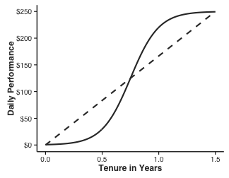
Figure 3. Performance Ramp Shapes
The Fully Ramped Performance Level
Some roles, such as Sales or Industrial Production, are more directly connected to revenue. When a Sales Rep makes a deal, a solid portion of the deal can be attributed to their work. When a Machinist builds a car door, it is not difficult to apportion their productivity to revenue. A management consultant will always have billable hours and rates high on their mind. Brief consultations with accounting or senior management can determine a percentage to allocate to each unit.
For example, perhaps we allocate 20% of a software sale’s value to the sales rep who sold the software. On an aggregate level, a sales group with 200 reps may sell $100M per year, so each rep is responsible for ($100M x 20% / 200 employees = $100,000) per rep per year, or $500 a day. In real life, reps’ performance differs – but we don’t know how a new rep will perform on their first day, so the average is our expected value.
Other roles, such as an Accountant, or a CEO, or a Software Developer, have a less tangible connection to the top line. There are two ways to estimate these. First, we can allocate a portion of revenue to each department, say Accounting, and divide by the number of employees. For example, ($100M x 1% / 20 accountants = $50,000) per accountant per year, or $250 per day.
Second, we can simply estimate a profit ratio based on salary. For example, we may estimate that the contribution is 20% over salary. So, a daily salary of $100 would imply a $120 daily contribution. For companies with unusually low revenue, this may be the only way to do it.
Ongoing Performance
The focus of this analysis is usually on attrition and the first years. But the approach can be extended to evaluate the contributions of long-tenured employees as well.
Several possible shapes are possible: – Employees may plateau at their full level – arguably a five-year underwriter may not be more productive than a two-year underwriter. – Employees may “dome” after the full level – after a certain level of tenure, they may not work as hard. – Employees may continue to learn, grow, and contribute – slowly ramping upwards forever.
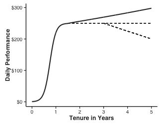
Figure 4. Long-Term Employee Performance Curves
The Final Performance Curve
The result of these three elements is a curve, much like the cost curve. For every day of tenure, we show a dollar contribution for a new employee in the role.
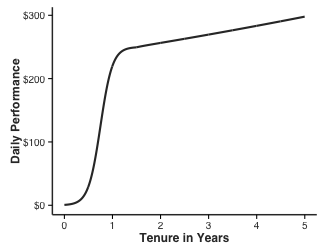
Figure 5. The Performance Curve
Human Resource Accounting
There is a sub-field of accounting called Human Resource Accounting (HRA) that delves more deeply into these valuations, rigorously treating employees as assets instead of costs. When scaled to the entire enterprise, HRA can be prohibitively complex. For a single role, we need not dig as deep – simple heuristics can build the curves very well.
Quantitative Scissors and The Hockey Stick: Net Employee Value
Now it is time to put the cost curve and the performance curve together.
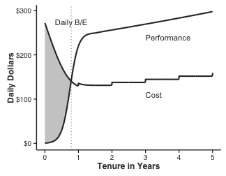
Figure 6. Cost and Performance for One Employee
Figure 6 shows a stylized cost/Performance plot for one employee across five years of tenure. At first, costs from recruiting, on-boarding, and training are high while performance is zero. Every day the employee comes in, the business loses money. At 9 months the lines cross – and for the first time, the employee delivers a net positive contribution. This is called the “Daily Breakeven Point.”
Beyond this point, a long-term pattern of net positive contribution endures. These crossing curves are sometimes called the “quantitative scissors” – the left “red zone” is an inescapable reality of doing business. To decrease the overall costs due to employee churn, something has to budge on these curves. However, daily breakeven is not the full story.
Cumulative Breakeven
We must account for the “debt” incurred by training and early costs. The cumulative sum of daily losses or surpluses brings us the “Cumulative Value” chart:
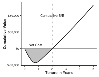
Figure 7. Cumulative Value for One Employee
The cumulative value generally falls into a familiar “hockey stick” shape as in Figure 7. The plot shows the net value accrued by an employee once they get to a specific tenure. It shows us when the “debt” from recruiting and training costs is paid off, and the line crosses zero. This point is called the “Cumulative Breakeven.”
The cumulative value curve is a valuable business object. The shaded region on the left shows how terminations before this point are a cost to the business.
In this stylized example, the employee starts providing daily value after 9 months, and does not pay back the startup “debt” until after 24 months. An employee who leaves at 9 months represents a net cost of over $25,000 in lost startup costs. By comparison, we often see impressive attrition after just 3-6 months.
In calculations that span into very long tenures, it may be advisable to adjust values for inflation.
Replacement Cost
When an employee must be replaced, the business has lost a functioning asset, a valuable team member. A proper replacement should be considered as a fully-trained, fully-ramped-up employee, ready to take on the work.
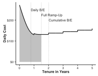
Figure 8. Replacement Cost Cutoffs
For such calculations we sum up the costs under the Cost Curve to one of three places, depending on internal policy:
We count the costs only, to identify the total additional outlay that the business is forced to make upon losing a staff member. The Full Productivity Point is the most intuitive, stable, and defensible option. This number is typically thousands of dollars even for entry-level positions.
In Part 3 Pasha will discuss Using Survival Analytics to Understand and Predict Employee Tenure.
Author Bio
 Pasha Roberts is chief scientist at Talent Analytics Corp., a company that uses data science to model and optimize employee performance in areas such as call center staff, sales organizations and analytics professionals. He wrote the first implementation of the company’s software over a decade ago and continues to drive new features and platforms for the company. He holds a bachelor’s degree in economics and Russian studies from The College of William and Mary, and a master of science degree in financial engineering from the MIT Sloan School of Management.