
Data science has a measurement problem. Simple metrics may not address complex situations. But complex metrics present myriad problems.
What is the best way to quantify the quality of your classification algorithm? As we strive for better algorithms, we often fail to think critically about what it means for predictions to be “good”. Evaluation methodology and decision theory are tightly linked. Often a classifier outputs numerical scores but a performance metric takes binary predictions. In these cases, any such metric specifies an optimal decision rule to convert scores to predictions. Thus in many settings, it would seem data scientists should consider how a system should behave when choosing a performance metric. Last September, at ECML in Nancy, I presented a paper exploring some surprising properties of F1 score. (full pdf) In this post, I’ll explore some of the deep problems our community faces as regards evaluation methodology.
Imagine you want to classify documents with binary labels. Perhaps you are trying to classify emails as spam/not spam. Or perhaps you have a collection of documents and a vocabulary of tags (as in a blog post like this) and want to apply the appropriate tags for each document. Formally, we call the spam detection problem binary classification and the autotagging problem multilabel classification.
So you choose your favorite classification algorithm, for instance logistic regression or a support vector machine. You regularize to maximize performance on holdout data. For simplicity, assume that in the multilabel case, a separate classifier is trained for each label. Finally, you have a model that can attach real valued scores to documents. You might think you’re done! But some glaring questions remain.
What do you do with these scores?
What does it mean for a system to output “good” scores?
How can you compare the performance of logistic regression, which minimizes log loss, against a support vector machine, which minimizes hinge loss?
Should a performance metric operate on real valued scores or binary predictions?
How does class balance influence the choice of performance metric?
If the dataset is multilabel, how do you aggregate scores across labels?
In both the research community and data science practice, a lot of thought goes into designing and optimizing algorithms, but too often evaluation methodology is an afterthought.
Evaluating Rankings vs. Predictions
A primary consideration is whether an evaluation metric should take as input ordinal rankings or binary predictions. In either case, it may be useful to first formalize a few terms. When the ground truth label is positive, we call this an actual positive. When the predicted label is positive, we call this a predicted positive. As indicated in the following confusion matrix (Figure 1), False positives and false negatives occur when the predicted label and ground truth disagree.

In an information theoretic sense, rankings are clearly more expressive than binary outputs. Given rankings, a user could impose their own cost-sensitivity (relative costs of false positive and false negative) and craft their own decision theory. Further, several established performance metrics exist which operate on rankings as inputs. Area under the ROC curve (AUROC) is one common metric that operates on fully specified rankings. AUROC plots the true positive rate against the false positive rate. A system that predicts all actual positives ahead of all actual negatives achieves the maximum AUROC score of 1. A system outputting completely random rankings would be expected to achieve an AUROC of .5. (An example AUROC taken from Wikipedia is shown below.) 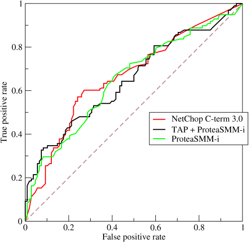
On the other hand, such a method requires dense predictions in order to evaluate their comparative worth. To evaluate the performance of a system on a multilabel dataset, one would need to submit as many predictions as there are examples times labels. Another drawback to evaluating performance based on rankings is that it may bias the evaluation against algorithms such as decision trees, which output 0/1 classifications but not rankings.
Binary Metrics – Accuracy
The most widely known metrics operate on binary predictions. In other words, if the model outputs numerical values, these must be thresholded to produce binary (positive/negative) predictions. Among the binary metrics, accuracy is the simplest. Expressible as (tp + tn) / N, where N is the total number of predictions, accuracy has several charming properties. For example, given scores which are calibrated probabilities, the threshold to maximize accuracy is simply .5. We’ll postpone a serious conversation on calibration for another post. But suffice it to say that a calibrated probability behaves like a real probability. If 1000 examples receive a score of .5 each, we expect roughly 500 of them to be positive. Another nice property of accuracy emerges in the multilabel case. The accuracy as calculated on the total confusion matrix across many labels is identical to averaging the accuracy calculated separately on each label.
One might reasonably wonder under what conditions we would ever want an alternative metric, given accuracy’s useful properties. However, class imbalance presents such a scenario. In many information retrieval tasks, the positive class is much rarer than the negative class. In these cases, when nearly all examples are actually negative, a trivial classifier that always predicts negative would get a great score, despite adding no information.
Binary Metrics – F1
For this reason, many researchers and data scientists report F1 score when working with unbalanced datasets. F1 score is the harmonic mean (a kind of average) of precision and recall. Precision, which can be expressed as tp / (tp + fp) is the percentage of all positive predictions that are in fact actual positives. Recall can be expressed as tp/(tp + fn) and captures the fraction of all actual positives that are predicted positive. F1 can then be expressed as 2tp / (2tp + fp + fn) and requires both high recall and high precision to yield a high score. This all might intuitively reasonable. What could possibly go wrong?
F1’s Definition Problem
First, it might have occurred when vieweing the definitions of precision and recall that recall is undefined when the number of actual positives is 0. Similarly precision is undefined when the number of positive predictions is 0. Further, when there are no actual positives and no examples are predicted positive, even the reduced expression of F1 is undefined. It’s unlikely that a test set for a single label binary classification will contain 0 actual positives. But when working with a large multilabel problem, such as autotagging news articles according to specific categories, some subset of categories may not be present in a test set. I know of no agreed upon convention which specifies the F1 score in these scenarios. Thus, on multilabel datasets, when the reported F1 score is the average F1 score across labels, It may be impossible to properly compare the self-reported scores from two different groups of researchers. Likely, many implementations set the undefined value to 1. Consider a classifier which predicts all examples to be negative. On a shuffle of the data with no actual positives, it may get an F1 Score of 1. But were there a single actual positive, it would get a score of 0!
F1’s Thresholding Problem
Recall the straight-forwardness of thresholding probabilistic output to maximize accuracy. Now consider F1. As we showed in our paper, the optimal threshold to convert real-valued scores to F1-optimal binary predictions is not straightforward. This is further evidenced by the considerable body of papers that address the task of choosing the optimal threshold. Most systems rely upon a “plug-in rule.” This means that first they learn a normal classifier and then feed the probabilistic predictions into an algorithm which decides the threshold.
While clearly many people optimize predictions before reporting F1 score, there is no reason to believe that everyone who reports F1 score optimizes their predictions. It is plausible that many researchers threshold at .5, reporting several metrics using those predictions, while other researchers separately threshold to maximize performance on each metric. Taken together, the definitional ambiguity and thresholding difficulty associated with F1 present formidable obstacles to comparing the results of competing systems.
Some important questions arise:
Does the system with the better score have a stronger underlying algorithm or simply cleverer thresholding?
While great F1 requires a great underlying classifier, how suitable are the decisions which maximize F1 for any real-world task?
What happens in the case when the underlying classifier is not so great?
In our paper we identified some simple but perhaps common pathological cases. One curious behavior is that regardless of how rare a label is, if the classifier is completely uninformative (predicts the same low score for every example), the way to maximize F1 is to predict every example to be positive! We encountered just such a problem on a large multilabel document classification task, when the only predictive feature for a rare label was lost to feature selection. As a result, our system tagged a large percentage of articles with the very rare label “platypus”. This appeared to be a bug, but was actually the optimal behavior given our poor classifier!
F1’s Multilabel Problem
Remember that one nice property of accuracy is that it is identical to calculate accuracy on a confusion matrix collected across all labels or to average the accuracy as separately calculated across all labels. Unfortunately, this is not the case for F1. Collecting a confusion matrix across all labels is called micro-F1, and results in one threshold across all labels. Macro-F1, on the other hand which averages F1 scores across labels results in setting a separate threshold for each label. Averaging F1 scores calculated separately on each example represents a third approach.
Addressing Cost Sensitivity
In a sense, any threshold implies a cost-sensitive setting. The optimal threshold to maximize F1 is always less than or equal to .5. Informally, we can say this means that when we use F1, we care more about false negatives than false positives. By using F1 score, we outsource the responsibility of choosing “how much more”. However, we could explicitly chose our relative costs, perhaps by looking to the problem domain for some intrinsic cost ratio. In these cases we could craft a weighted version of accuracy, salvaging the benefits of a linear performance metric.
Wrap-up
Evaluating machine learning algorithms in the setting of class imbalance is a deep problem, which is complicated further in the multilabel setting. When, like F1, a metric has definitional ambiguity, comparing self-reported performance across different systems can be impossible even when researchers are honest and well-intentioned. Further, when a metric is difficult to threshold optimally, it may be difficult to determine which system produced the most informative scores and which went about thresholding more meticulously. Because data-mining research papers often don’t decribe thresholding strategy, this problem is even more confounding. While algorithms may be more exciting than evaluation methodology, it behooves the data science community to think critically about how machine learning systems will be used and to choose evaluation metrics which imply appropriate decision theory.
Zachary Chase Lipton is a PhD student in the Computer Science Engineering department at the University of California, San Diego. Funded by the Division of Biomedical Informatics, he is interested in both theoretical foundations and applications of machine learning. In addition to his work at UCSD, he has interned at Microsoft Research Labs.